Data science is an evolutionary extension of statistics capable of dealing with the massive amounts of data that are regularly produced today. It adds methods from computer science to the repertoire of statistics.

Data scientists who need to work with data for analysis, modeling, or forecasting should become familiar with NumPy’s usage and its capabilities, as it will help them quickly prototype and test their ideas. This article aims to introduce you to some basic fundamental concepts of NumPy, such as:
Let’s get started.
NumPy, short for Numerical Python, provides an efficient interface for storing and manipulating extensive data in the Python programming language. NumPy supplies functions you can call, which makes it especially useful for data manipulations. Later in this article, we will look into the methods and operations we can perform in NumPy.
In one way or another, a NumPy array is like Python’s inbuilt list type, but NumPy arrays offer much more efficient storage and data operations as the dataset grows larger. NumPy offers a special kind of array that makes use of multidimensional arrays, called ndarrays, or N-dimensional arrays.
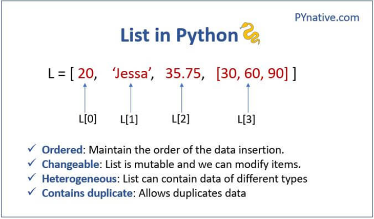
An array is a container or wrapper that has a collection of elements of the same type, and can be one or more dimensions. A NumPy array is also homogenous — i.e., it contains data of all the same data type.
As data scientists, the dimension of our array is essential to us, as it will enable us to know the structure of our dataset. NumPy has an inbuilt function for finding the dimension of the array.
A dimension of an array is a direction in which elements are arranged. It is similar to the concept of axes and could be equated to visualizing data in x-, y-, or z-axes etc., depending on the number of rows and columns we have in a dataset.
When we have one feature or column, the dimension is a one-dimensional array. It is 2D when we have two columns.

A vector is an array of one dimension. We have a single vector when our dataset is meant to take a single column of input and is expected to make predictions from it.
Data scientists constantly work with matrices and vectors; however, whenever we have many features in our dataset, and we end up using only one of the features for our model, the dimension of the feature has changed to one, which makes it a vector.
Below is a sample dataset. Our inputs/features are x1 and x2 while output/target is y.
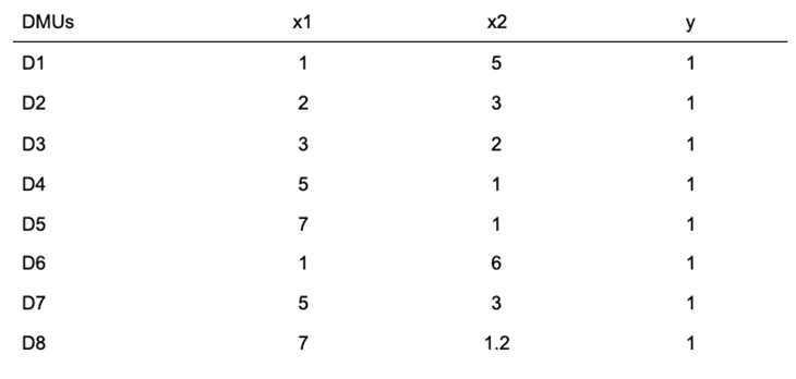
If we selected the x1 feature for our model, then we have a vector of a one-dimensional array. But, if we have x1 and x2 features, then we have a matrix, or a 2-dimensional array.
python
import numpy as np
x1 = np.array([1,2,3,5,7,1,5,7])
x2 = np.array([5,3,2,1,1,6,3,1.2])
x1
print(x2)
A matrix is an array of two dimensions and above. As data scientists, we may encounter a state where we have a dataset with single input and single output columns. Therefore, our array has more than one dimension, and then it is called a matrix of x and y-axis. In this case, we say our array is n-dimensional.
This is a matrix of a 2D array, and here we have x- and y-axes.
| 1 | 2 | 3 | 4 | 5 |
| 4 | 3 | 4 | 3 | 4 |
This is a matrix of a 3D array with three axes: x, y, and z.
| 1 | 2 | 3 | 4 | 5 |
| 4 | 3 | 4 | 3 | 4 |
| 0 | 3 | 5 | 9 | 6 |
All ndarray elements are homogeneous — meaning they are of the same data type, so they use the same amount of computer memory. This leads us to the concept of type promotion and data types in NumPy.
Type promotion is a situation where NumPy converts any element from one data type to another.
In the diagram below, there is a mix of numbers in different data types, float and int. The result will give us the same number if they are in the Python list format.
| 1.2 | 2 | 3 | 4 | 5 |
If we had a Python list with int and float types, nothing would change here.
| 1.2 | 2 | 3 | 4 | 5 |
| 1.2 | 2 | 3 | 4 | 5 |
But unlike a Python list, a NumPy array interacts better with elements of the same type. Let’s see how this plays out in practice.
NumPy promotes all the arrays to a floating-point number. This diagram is the result of converting the NumPy array to this data type.
| 1.2 | 2 | 3 | 4 | 5 |
| 1.2 | 2.0 | 3.0 | 4.0 | 5.0 |
In the code sample below, we created a Python list. Next, we shall make a NumPy array of this combination of two different types of elements — i.e., integers and floats.
python
import numpy as np
pythonList = [1,2,3,3.3]
numpyArray = np.array(pythonList)
print("all elements promoted to",numpyArray.dtype)

Result;
all elements promoted to float64
Using the dtype function in NumPy, the type of elements in the array are promoted to float64. It emphasizes that the NumPy array prioritizes floats above integers by converting the entire array of integers to floats.
The code sample below combines a list of integers with a list of strings and then promotes them all to Unicode string. It implies that the string has a higher priority over the integers.
python
import numpy as np
pythonList = [1,2,3,'t']
print(pythonList)
numpyArray = np.array(pythonList)
print(numpyArray.dtype)

We get this result:
[1, 2, 3, 't']
<U21
Understanding the concept of type promotion will guide us through what to do when we have type errors while working with NumPy. In the code sample below, we have a type error:
python
import numpy as np
pythonList = [1,2,3,'t']
print(pythonList)
numpyArray = np.array(pythonList)
print(numpyArray + 2)

UFuncTypeError: ufunc 'add' did not contain a loop with signature matching types (dtype('<U21'), dtype('<U21')) -> dtype('<U21')
Which means that, when elements are promoted to a Unicode string, we cannot perform any mathematical operations on them.
Before we get started, make sure you have a version of Python that’s at least ≥ 3.0, and have installed NumPy ≥ v1.8.
Working with NumPy entails importing the NumPy module before you start writing the code.
When we import NumPy as np, we establish a link with NumPy. We are also shortening the word “numpy” to “np” to make our code easier to read and help avoid namespace issues.
python
import numpy as np

The above is the same as the below:

python
import numpy
np = numpy
del numpy
The standard NumPy import, under the alias np, can also be named anything you want it to be.
The code snippet below depicts how to call NumPy’s inbuilt method (array) on a Python list of integers to form a NumPy array object.
python
import numpy as np
pyList = [1,2,3,4,5]
numpy_array = np.array(pyList)
numpy_array
array functionWe can import the array() function from the NumPy library to create our arrays.
python from numpy import array arr = array([[1],[2],[3]]) arr
zeros and ones function to create NumPy arraysAs data scientists, we sometimes create arrays filled solely with 0 or 1. For instance, binary data is labeled with 0 and 1, we may need dummy datasets of one label.
In order to create these arrays, NumPy provides the functions np.zeros and np.ones. They both take in the same arguments, which includes just one required argument — the array shape. The functions also allow for manual casting using the dtype keyword argument.
The code below shows example usages of np.zeros and np.ones.
python
import numpy as nd
zeros = nd.zeros(6)
zeros
Change the type here:
python
import numpy as np
ones_array = np.ones(6, dtype = int)
ones_array
We can alternative create a matrix of it:
python
import numpy as np
arr = np.ones(6, dtype = int).reshape(3,2)
arr
In order to create an array filled with a specific number of ones, we’ll use the ones function.
python import numpy as np arr = np.ones(12, dtype = int) arr Matrix form python import numpy as np arr = np.ones(12, dtype = int).reshape(3,4) arr
We can as well perform a mathematical operation on the array:
This will fill our array with 3s instead of 1s:
python
import numpy as np
ones_array = np.ones(6, dtype = int) * 3
ones_array
dtype attributeWhile exploring a dataset, it is part of the standard to familiarize yourself with the type of elements you have in each column. This will give us an overview of the dataset. To learn more about the usage of this attribute, check the documentation.
The dtype attribute can show the type of elements in an array.
python
import numpy as nd
find_type1 = nd.array([2,3,5,3,3,1,2,0,3.4,3.3])
find_type2 = nd.array([[2,3,5],[3,5,4],[1,2,3],[0,3,3]])
print("first variable is of type", find_type1.dtype)
print("second variable is of type", find_type2.dtype)
In order to have more control over the form of data we want to feed to our model, we can change the type of element in our dataset using the dtype property.
However, while we can convert integers to floats, or vice versa, and integers or floats to complex numbers, and vice versa, we cannot convert any of the data types above to a string.
Using the dtype function in NumPy enables us to convert the elements from floats to ints:
python
import numpy as nd
ones = nd.ones(6,dtype = int)
ones

Result;
array([1, 1, 1, 1, 1, 1])

python
import numpy as nd
arr = nd.array([[2,3,5],[3,5,4],[1,2,3],[0,3,3]],dtype = float)
print("the elements type  is", arr.dtype)
type and dtype attributesThe type belongs to Python. It unravels the type of Python data type we are working with. Visit the documentation for more on Python data types.
Using type in the code sample below shows us that we have a special Python object, which is numpy.ndarray. It is similar to how type("string") works for Python strings; for example, the code sample below displays the type of the object.
python
import numpy as np
arrs = np.array([[2,4,6],[3,2,4],[6,4,2]])
type(arrs)
The dtype property, on the other hand, is one of NumPy’s inbuilt properties. As we explained earlier, NumPy has its own data types that are different from Python data types, so we can use the dtype property to find out which NumPy data type we are working with.
Below, we shall use NumPy’s dtype property to find out which type of elements are in our NumPy array.
import numpy as np
arrs = np.array([[2,4,6],[3,2,4],[6,4,2]])
arr.dtype
Any attempt to use the dtype attribute on another non-NumPy Python object will give us an error.
python
import numpy as np
pyList =[ "Listtype",2]
pyList.dtype
Result;
---------------------------------------------------------------------------
AttributeError Traceback (most recent call last)
<ipython-input-19-2756eacf407c> in <module>
1 arr = "string type"
----> 2 arr.dtype
AttributeError: 'list' object has no attribute 'dtype'
NumPy arrays are rich with a number of inbuilt functions. In this section, I will introduce you to the functions we’d use most often while working on datasets:
The reshape function will enable us to generate random data. It is not only good for rendering arrays to the columns and rows we want, but can also be helpful in converting a row to a column to row. This gives us the flexibility to manipulate our array the way we want it.
In the code snippet below, we have a vector, but we reshape it to a matrix, with an x-dimension and a y-dimension. The first argument in the reshape function is the row, and the second is the column.
We can use reshape to render our array in the desired shape we want to achieve. This is one of the wonders of NumPy.
python
import numpy as np
a = np.arrange(12)
matrix = a.reshape(3,4)
print(matrix)
We can also turn a row into a column or a column into a row. This makes the NumPy array more flexible to use for data manipulation.
python
import numpy as np
a = np.arrange(12)
vertical = a.reshape(12,1)
print(vertical)
The code snippet below starts with a one-dimensional array of nine elements, but we reshape it to two dimensions, with three rows and three columns.
python
import numpy as np
one_d_array = np.array([2,3,4,5,6,7,8,9,10])
reshaped_array = one_d_array.reshape(3,3)
reshaped_array
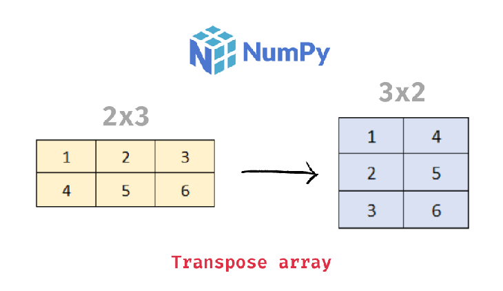
Just as reshaping data is common during data preprocessing, transposing data is also common. In some cases, we have data that’s supposed to be in a particular format, but receive some new data that is not in tandem with the data we have. This is where transposing the new data emerges to resolve the conflicting structure of our data.
We can just transpose the data using the np.transpose function to convert it to the proper format that fits the required data.
python
import numpy as np
arr = np.arrange(12)
arr = np.reshape(arr, (4, 3))
transposed_arr = np.transpose(arr)
print((arr))
print('arr shape: {}'.format(arr.shape))
print((transposed_arr))
print('new transposed shape: {}'.format(transposed_arr.shape))
Transpose wouldn’t work for a one-dimensional array:
import numpy as np
arr = np.arrange(12)
arr.ndim
transposed_arr = np.transpose(arr)
print((arr))
It is sometimes important to know the dimensions of our data during preprocessing. Performing mathematical operations on vectors and matrices with no similar dimensions will result in an error. For example, we can get an error from multiplying a 2D array by a 1D array.
If you don’t know the dimensions of your data, you can use the ndim attribute to find out.
python
import numpy as np
one_d_array = np.array([2,3,4,5,6,7,8,9,10])
reshaped_array = one_d_array.reshape(3,3)
reshaped_array.ndim
Using different dimensions gave the error below, hence the importance of knowing the dimensions of our arrays.
python import numpy as np one_d_array = np.array([2,3,4,5,6,7,8,9,10]) reshaped_array = one_d_array.reshape(3,3) reshaped_array * one_d_array Result; ValueError: operands could not be broadcast together with shapes (3,3) (9,)
More specifically, you can use the shape property to find the number of rows and columns in your array. Imbalances in the shapes can also give us errors when dealing with two different datasets. The code snippet shows how to find the shape of an array:
python
import numpy as np
one_d_array = np.array([2,3,4,5,6,7,8,9,10])
reshaped_array = one_d_array.reshape(3,3)
reshaped_array.shape
arrange and reshape functionsWith NumPy, we can easily generate numbers and use reshape functions to convert the numbers to any possible rows and columns we want. For example in the code sample below, the arrange function generates a single row of 1 to 13, while the reshape function renders the array to three rows and four columns.
python
import numpy as np
matrix =  np.arrange(1,13).reshape(3,4)
matrix
Data scientists mostly work with vectors and matrices while trying to perform data mining. In order to avoid errors during the preprocessing stage, it is crucial we check our arrays’ dimensions, shapes, and dtypes.
If we didn’t, we would get errors if we tried to perform mathematical operations on these matrices and vectors when their sizes, dimensions, and shapes are not the same.
Checking the dtype is to avoid type errors, as I explained in the previous section. But knowing each array’s dimensions and shape safeguards us from getting value errors.
For an overview of data preprocessing, kindly check this HackerNoon post.
Below is an example of two-vector arithmetic:
python
from numpy import array
x1 = array([20,21,22,23,24])
x2 = array([21,23,2,2,3])
x1*x2
We can divide as well:
python
from numpy import array
x1 = array([20,21,22,23,24])
x2 = array([21,23,2,2,3])
x1/x2
Subtraction of two vectors looks like this:
python
from numpy import array
x1 = array([20,21,22,23,24])
x2 = array([21,23,2,2,3])
x1-x2
This is similar to performing any other mathematical operation, such as subtraction, division, and multiplication.
The addition of two vectors follows this pattern:
z = [z1,z2,z3,z4,z5]
y = [y1,y2,y3,y4,y5]
z + y =  z1 + y1, z2 + y2, z3 + y3, z4 + y4, z5 + y5

python
from numpy import array
z = array([2,3,4,5,6])
y = array([1,2,3,4,5])
sum_vectors = z + y
multiplication_vectors = z * y
sum_vectors
print(multiplication_vectors)
You can also perform mathematical operations on matrices:
import numpy as np
arr = np.array([[1, 2], [3, 4]])
# Square root element values
print('Square root', arr**0.5)
# Add 1 to element values
print('added one',arr + 1)
# Subtract element values by 1.2
print(arr - 1.2)
# Double element values
print(arr * 2)
# Halve element values
print(arr / 2)
# Integer division (half)
print(arr // 2)
# Square element values
print(arr**2)
sum function in NumPyIn the previous section on mathematical operations, we summed the values between two vectors. There are cases where we can also use the inbuilt function (np.sum) in NumPy to sum the values within a single array.
The code snippet below shows how to use np.sum:
If the np.sum axis is equal to 0, the addition is done along the column; it switches to rows when the axis is equal to 1. If the axis is not defined, the overall sum of the array is returned.
python
import numpy as np
sum = np.array([[3, 72, 3],
[1, 7, -6],
[-2, -9, 8]])
print(np.sum(sum))
print(np.sum(sum, axis=0))
print(np.sum(sum, axis=1))
Result;
77
[ 2 70 5]
[78 2 -3]
NumPy is also useful to analyze data for its main characteristics and interesting trends. There are a few techniques in NumPy that allow us to quickly inspect data arrays. NumPy comes with some statistical functions, but we’ll use the scikit-learn library — one of the core libraries for professional-level data analysis.
For example, we can obtain the minimum and maximum values of a NumPy array using its inbuilt min and max functions. This gives us an initial sense of the data’s range and can alert us to extreme outliers in the data.
The code below shows example usages of the min and max functions.
python
import numpy as np
arr = np.array([[0, 72, 3],
               [1, 3, -60],
               [-3, -2, 4]])
print(arr.min())
print(arr.max())

print(arr.min(axis=0))
print(arr.max(axis=-1))

Result;
-60
72
[ -3  -2 -60]
[72  3  4]
Data scientists tend to work on smaller datasets than machine learning engineers, and their main goal is to analyze the data and quickly extract usable results. Therefore, they focus more on the traditional data inference models found in scikit-learn, rather than deep neural networks.
The scikit-learn library includes tools for data preprocessing and data mining. It is imported in Python via the statement import sklearn.
This computes the arithmetic mean along the specified axis:
mean(a[,axis,dtype,keepdims,where])
This finds the standard deviation in a dataset:
std(a[, axis, dtype, out, ddof, keepdims, where])
An index is the position of a value. Indexing is aimed at getting a specific value in the array by referring to its index or position. In data science, we make use of indexing a lot because it allows us to select an element from an array, a single row/column, etc.
While working with an array, we may need to locate a specific row or column from the array. Let’s see how indexing works in NumPy.
The first position index is denoted as 0 which represents the first row.
python
import numpy as np
matrix =  np.arrange(1,13).reshape(3,4)
matrix[0]

Now, let's try getting the third row from the array.
python
import numpy as np
matrix[2]
The below gives us a vector from the last row.
python
import numpy as np
matrix[-1]
Every element, row, and column have an array index position numbering from 0. It can also be a selection of one or more elements from a vector.
This is as simple as trying to filter a column or rows from a matrix. For example, we can select a single value from several values in the below example. The values are numbered sequentially in the index memory, starting from zero.
| index | 0 | 1 | 2 | 3 |
| value | 2 | 4 | 5 | 10 |
For instance, getting a value at index 0 will give us 2, which is a scalar.
python
import numpy as np
value =  np.array([2,4,5,10])
value[0]
A matrix is more like an array of vectors. A single row or column is referred to as a vector, but when there is more than one row, we have a matrix.
We are getting the position of vectors in the matrix below using square brackets.
| vector[0] | 1 | 2 | 3 |
| vector[1] | 4 | 5 | 6 |
| vector[2] | 7 | 8 | 9 |
| vector[3] | 10 | 11 | 12 |
vector[0] => [1,2,3]
vector[1] => [4,5,6]
vector[2] => [7,8,9]
vector[3] => [10,11,12]
Getting an element of vector[0] is done by adding the index of the element.
vector[0,0] => 1
vector[0,1] => 2
vector[0,2] => 3
This gives us a scalar or element of the second position in the third row.
python
import numpy as np
matrix[2,1]
This selects the first column:
python
import numpy as np
matrix[:,0]
Select the second column:
python
import numpy as np
matrix[:,1]
This gets the last column:
python
import numpy as np
matrix[:,-1]
In this article, we learned about the fundamentals of NumPy with essential functions for manipulating NumPy arrays. I hope this helps you gain a basic understanding of Python on your path to becoming a data scientist.
Install LogRocket via npm or script tag. LogRocket.init() must be called client-side, not
server-side
$ npm i --save logrocket

// Code:

import LogRocket from 'logrocket';
LogRocket.init('app/id');
// Add to your HTML:

<script src="https://cdn.lr-ingest.com/LogRocket.min.js"></script>
<script>window.LogRocket && window.LogRocket.init('app/id');</script>

Discover how to build, render, and automate product demo videos with Remotion, replacing traditional screen recordings with reusable React code.

Chrome’s Modern Web Guidance embeds modern web platform skills into AI coding agents, helping them choose native HTML, CSS, and browser APIs over legacy patterns.

Learn how to use Fallow to analyze AI-generated code, detect dead code, duplicate logic, and complexity issues, and integrate automated code quality checks into your AI-assisted development workflow.

Learn how to protect full-stack projects from NPM supply chain attacks with a practical security checklist.
Hey there, want to help make our blog better?
Join LogRocket’s Content Advisory Board. You’ll help inform the type of content we create and get access to exclusive meetups, social accreditation, and swag.
Sign up now