
One of the most common ways of achieving visual variety is using procedural noise. Given its ability to add intricate details with low memory and manual costs, procedural noises are of great importance to the field of computer graphics, and their use is widespread throughout the industry.
In this article, we discuss two approaches for using procedural noises in Unity, as well as how they can be used to achieve a multitude of results and outcomes. The first is a code approach to procedural noise based on the Unity Mathematics package. This method is ideal for when you want to control the noise parameters, and their results in applications that are either not entirely visual or that will feed other algorithms, such as Prefab Spawners.
The second one is based on using Shader Graph nodes to use procedural noise in shaders. This approach is more suitable for Unity users who are familiar with visual coding and are looking for visual results using custom shaders. It is important to note that this approach requires the use of either the Universal Render Pipeline or the High-Definition Render Pipeline to enable the Shader Graph tools.
The Replay is a weekly newsletter for dev and engineering leaders.
Delivered once a week, it's your curated guide to the most important conversations around frontend dev, emerging AI tools, and the state of modern software.
Procedural noise, or simply noise, has been used in the industry for many processes, including clouds, waves, animation, and so on. In computer graphics, noise is a random, unstructured pattern without evident structure. Procedural noise describes a process in which we can procedurally generate noise patterns given a set of inputs.
Notice that noise is described as an unstructured pattern and is usually sought for these characteristics. That is because the pattern-like feature allows us to use it to convey detail and familiarity without presenting a straightforward design. Clouds, as mentioned before, have a clear visual identity but are not immediately clear about how their shapes are formed by just staring at them.
One of the most basic approaches to noise is white noise: a random collection of values from a range in which every possible value has equal chances of appearing.
In more accessible terms, generating white noise is like filling in a list of values, in which we throw a die for each value. All values from a die have the same probability, implying that they have equal chances of appearing. The image below illustrates what a 2D white noise image looks like:
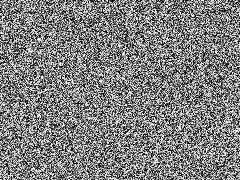
Its highly unpredictable behavior is both an advantage and a disadvantage of white noise. It is advantageous because it can quickly add variation to our process with a very low clear structure (or no clear structure at all). White noise is a good candidate if we want to portray dust or stars, for example.
But white noise is a disadvantage if we aim to model noise-like patterns like the ones cited previously. It is too chaotic to resemble clouds, for instance. For that, we resort to using other sources of noise.
In general, instead of referring to using noise directly, we use the term noise function, which is a process that results in a noise value. A white noise function could be written as:
float whiteNoiseFunction(float minimalValue, float maximalValue) {
    return Random.Range(minimalValue, maximalValue);
}
Or, for a Unity-like noise function to generate a 2D point:
Vector2 white2DNoiseFunction(float minimalValue, float maximalValue) {
    return new Vector2(Random.Range(minimalValue, maximalValue),
                                           Random.Range(minimalValue, maximalValue));
}
Luckily, Unity already has many implementations for noise functions that we can use to generate our noise values.
For starters, a Unity project has direct access to one of the more famous noise functions used in the industry: the Perlin Noise Function. An example of what a Perlin noise looks like can be seen below:
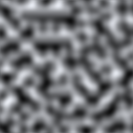
The Perlin Noise Function does not generate random numbers for all its positions. Instead, it divides the space into cells, forming a grid. Random numbers are generated at the edges of the grid, and the values within the cells are interpolated according to their proximity to the closest edges. That creates the wave-like pattern in which values increase and decrease across space.
The Perlin Noise Function implementation can be easily expanded from 2D to 3D and so on (for whatever reason you might need that).
We can access the Perlin Noise Function in Unity directly from the Mathf library. It has the following signature:
public static float PerlinNoise(float x, float y);
Since the Perlin Noise Function is based on a grid, its Unity implementation does not have a traditional implementation of one dimension (1D). However, that can be easily achieved by managing the inputs used. For example, the documentation suggests that simply using 0 as one of the arguments is an easy alternative to generating a 1D Perlin noise value.
Due to being accessible by default, the Mathf implementation of the Perlin Noise Function might be the most commonly seen noise function used in Unity tutorials. However, more noise function implementations can be accessed in Unity by importing the Mathematics package.
Unity’s Mathematics package encompasses efficient vector types and math functions with a shader-like syntax. As of the writing of this article, the Mathematics library was still considered a work in progress and should be used with care.
The package can be downloaded and imported to your project using the Package Manager. Select the option for the packages under Unity Registry, then select the Mathematics package, as seen in the image below:

The Mathematics noise functions are available as methods of the base Noise class. The noise functions available can be divided into four main groups, which are:
float2 cellular2x2 (float2 p)float cnoise (float2 p)float snoise (float2 v)float3 psrdnoise (float2 pos, float2 per, float rot)Except for the Perlin Noise Function, which was already covered previously, let us take a better look at these other functions and their usage in code. But, before that, it is crucial to understand how we can convert and work with the different data types used by the Mathematics package and Unity’s default variable types.
The Mathematics package uses other data types than the regular ones used by Unity. For example, instead of using Vector2, it uses float2. The core difference between them is that the Mathematic datatypes are specially designed for better performance and, as stated before, to better match with shader-like programming languages.
Although it is unclear whether Unity will phase out the older data types completely, for now, using both types is valid (not necessarily recommended), and the conversion between types is straightforward due to their similar data structures.
For example, converting a float2 to a Vector2 works as simple as:
float2 f2 = new float2(2.0f, 3.0f);
Vector2 v2 = (Vector2) f2;
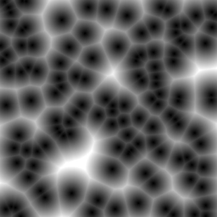
As stated previously, these functions are based on the Worley Noise Function, which itself is based on the Perlin Noise Function. In simple terms, the Worley Noise Function generates random points across a surface. Then, it calculates the value of individual points on this surface by interpolating its value toward the closest random point to it.
Due to this process, the resulting image resembles a cellular (hence the other name) structure. The image below provides an example of a resulting 2D image built by using the Worley Noise Function.
There are many variations in the package’s cellular functions, which vary from dimensionality (either 2D or 3D) and efficiency (lesser precision for the sake of speed). The cellular function receives a float2 as a parameter for the x and y position and returns the corresponding noise value for it. The more performance friendly version of this function is the cellular2x2 function, which has the same signature and use.
From a basic test comparison, the cellular2x2 is about three times faster in execution compared to the cellular counterpart.
N.B., the test was done by executing each noise function 100.000 using the same x and y parameters and measuring the total time spent.
Simplex noise functions were originally developed by Ken Perlin, the same developer of the original Perlin Noise Function. It is computationally more efficient than the Perlon Noise Function and is better suited for more dimensions (such as 4 and 5 dimensions). Moreover, the simplex noise function has less noticeable visual artifacts when compared to the original function.
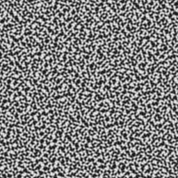
As for the others, many variations for the Simplex Noise Function are available in the package, which vary in dimensionality (from 2D, 3D, and 4D). All the functions share the same name, snoise, and differ from the available parameters. The 2D call for a simplex noise function takes a float2 as a parameter for the x and y positions and returns the corresponding noise value.
Oddly enough, in a basic test comparing the Simplex Noise Function (snoise) and the Mathematics package implementation of the Perlin Noise Function (cnoise), the Perlin functions for 2D and 4D values were about 24 and 42 percent, respectively, faster than the simplex function.
N.B., the test was done by executing each noise function 100.000 using the same x and y parameters and measuring the total time spent.
The Mathematics library also contains other methods besides the ones we just discussed, which are variations by adding new parameters to control their results. For example, the library contains a psdrnoise function, which takes 3 parameters: a float2 for the position, another float2 for the tiling, and a float value for the rotation. Due to their niche usage, this article will not focus further on them.
If you want to read more about them, I suggest you check their source codes in the repository and read this thread at the Unity forum. Moreover, feel free to drop a comment if you want an article on the topic. 😉
Accessing noise functions via code allows us to use their values directly in our functions, as opposed to having them calculated into an intermediary structure (a texture, for example). Thus, these functions are also good substitutes for randomizers.
Let’s say, for example, that you want to distribute some prefabs in a scene (a Prefab Spawner). We could achieve it by using the following code:
public void SpawnPrefab(Vector3 position, float frequency, float radius)
{
   //Generates a random point within a given radius
   var randomPosition = Random.insideUnitSphere * radius;
   //Add the original position
   randomPosition.x += position.x;
   randomPosition.y += position.y;
   randomPosition.z += position.z;

   //Only instantiates the prefab if it is within a certain noise frequency. For this case, we are using the position itself as the noise function parameter.
   if (noise.snoise(position) <= frequency)
   {
       Instantiate(prefab, randomPosition, Quaternion.identity);
   }
}
Another useful approach for noises via code is to procedurally generate textures through them. It is possible to perform these steps via code. However, for that, we have an easier and more flexible alternative.
Shader Graph is a Unity tool that allows users to visually program shaders with a node-based system. It enables fast and visual iterations while designing shaders. Moreover, even though it is node-based, Shader Graph has specific nodes that allow the user to write shader language as a text, string, or load shader HLSL code.
To access the Shader Graph tool, your application needs to be in either the Universal Render Pipeline or the High Definition Render Pipeline. Shaders can be created by accessing the menus Asset > Create > Shader Graph.
Shaders can be edited in the Shader Graph window, which displays the functionalities for parameters, previews, and outputs. This window is used to design the shader through connecting nodes.
Due to its complexity, the Shader Graph tool itself is not going to be covered by this article, except for some of its functionalities related to working with the Noise nodes. For more information on how to get started with the Shader Graph tool, refer to this other article.
By default, the Shader Graph tool has three nodes for noises, which are the Gradient Noise, the Simple Noise, and the Voronoi Noise. The image below shows all of these nodes with their respective previews and default values.
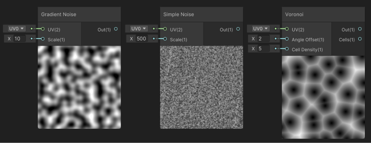
Let us discuss them one by one and compare them to the noise functions discussed before:
Similarly to the Mathematics package, these noise functions receive coordinates as parameters. The main difference is that these nodes automatically assign the UV coordinate as input for the noise function coordinates, which can be easily changed to any other type of two-dimensional vector.
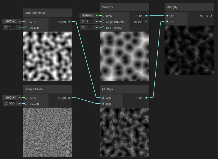
A common approach to these noises is combining them by performing simple mathematical operations, such as summing and multiplying their values. The image below shows the result of multiplying these three noises in sequence.
As stated at the end of the last section, we can use the Mathematics package to generate noise values via code and use them on our systems to control aspects. Alternatively, we use the Shader Graph tool to generate noise values via nodes and use them visually in our materials and other visual elements, such as particle systems and trail renderers.
Indeed you can mix both of them and use them for each other’s purposes, but this approach might be counterproductive. I recommend you stick to the rule of thumb of “code for code, visuals for visuals.”
Combining simple nodes is easy and fast to achieve a wide range of outcomes. For example, due to its interpolation between values, both the Gradient Noise node and the Simple Noise node are good candidates to make a simple cloud shader:
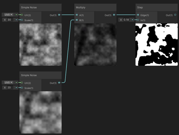
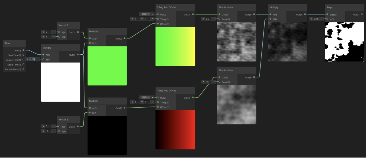
By multiplying Simple Noise nodes with varying scales, we further break the noise-generated structure. The result is then used in a Step node, which given an input returns 1 if it is higher than the input variable or 0 otherwise.
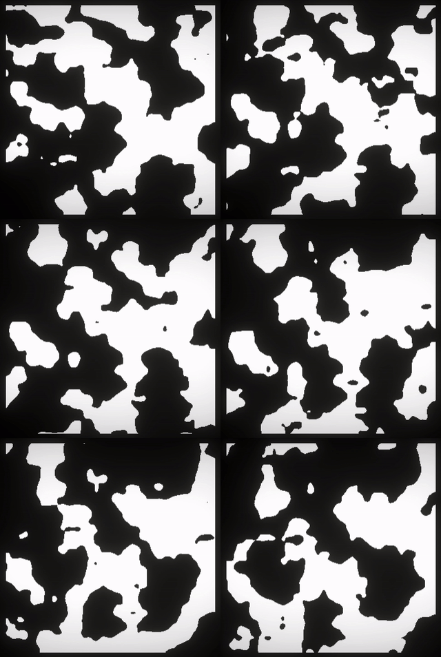
The following image shows an extension of this given graph for an animated version of the cloud pattern achieved by offsetting the UVs from both Simple Noise nodes in opposing directions:
The GIF below shows the animated result:
Although only partially related to this topic, a combination of nodes is often repeated for many Shader Graphs that use noises: animating the UVs by offsetting their values over time.
We have seen its usage on the previous graph for a cloud-like pattern. Still, it deserves a brief explanation since it is commonly used in many other implementations of animated noise patterns.
The graph below shows the necessary nodes to achieve this:
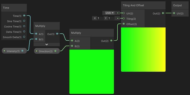
We use the Offset parameter to move the UV by a given value in x and y. The offset value is calculated using the Time node, multiplied by an Intensity value which helps us control how fast/slow we want the movement.
The result is then used to multiply a Vector2 for which direction we want to offset the UV. If we want a horizontal movement, we use a Vector with x = 1 and y = 0, while a vertical movement would use a vector x = 0 and y = 1.
Other combinations are possible, but if the directional vector’s magnitude is not 1 (i.e., the directional vector is not unitary), it will affect the intensity and cause your movement to be either faster or slower than initially expected. To safeguard against this issue, you can use a Normalize node after the Multiply node and connect its output to the Tiling and Offset node.
For simplicity, the coming Shader Graphs will use this graph as a Sub Graph. This Sub Graph, named UVOffsetOverTime, takes two float parameters: Intensity and Direction. Its output is a Vector2 for the newly calculated UV.
Furthermore, it is noticeable that this Sub Graph uses the default UV0 for the Tiling and Offset node. If that is not your (main) intention, you can also easily add a third parameter to it to pass the UV to the graph.
Using these same ideas, we can quickly sketch other effects, such as a water shader:
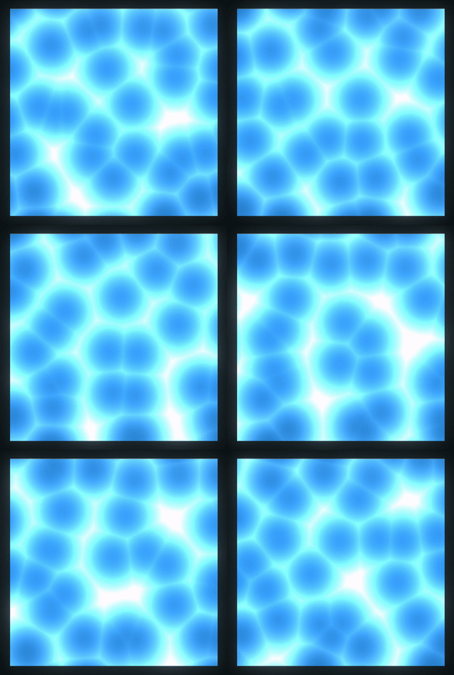
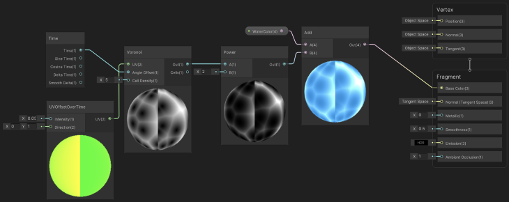
In this case, we are also using the Time node to change Voronoi’s Angle Offset parameter. This way, the internal points for the Voronoi Noise Function will also move, which creates a cellular-like motion characteristic of liquids such as water and lava surfaces.
On the other hand, to break the visual appearance of cells, the result of the Voronoi node is used in a Power node, which emphasizes higher values (closer to 1) and reduces lower values (closer to 0).
Also, as an example of a shader that uses all three of these noise nodes for different functions, we can build a Lava shader such as this:
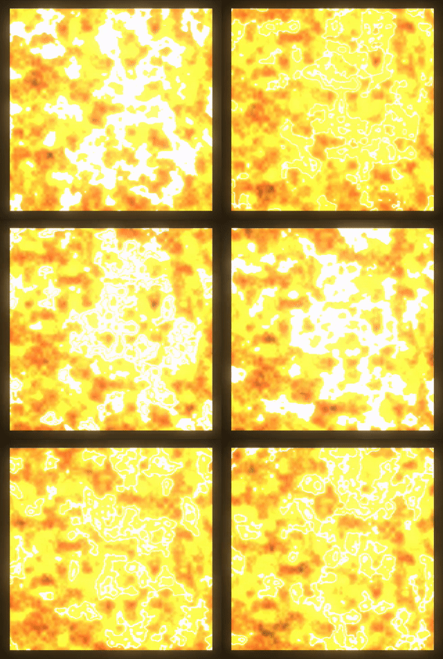
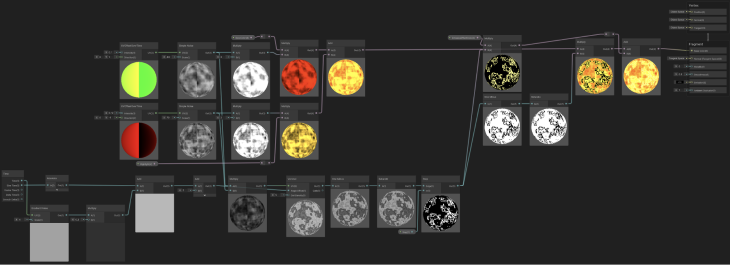
As you can see above, the lava shader has considerably more nodes than our simple water shader. Let us see it in parts to understand how the noise nodes were applied to achieve the final result.


To start, we use the UVOffsetSubGraph twice, with opposing directional vectors, to control two Simple Noise nodes. The two Simple Noise nodes have different scales to create enough difference between them, as we will combine their results later, similar to what was done for the Cloud Graph.
Moreover, to strengthen the noise values before multiplying them with a color, both results of the Noise nodes are multiplied by 2. This process brightens up the result.
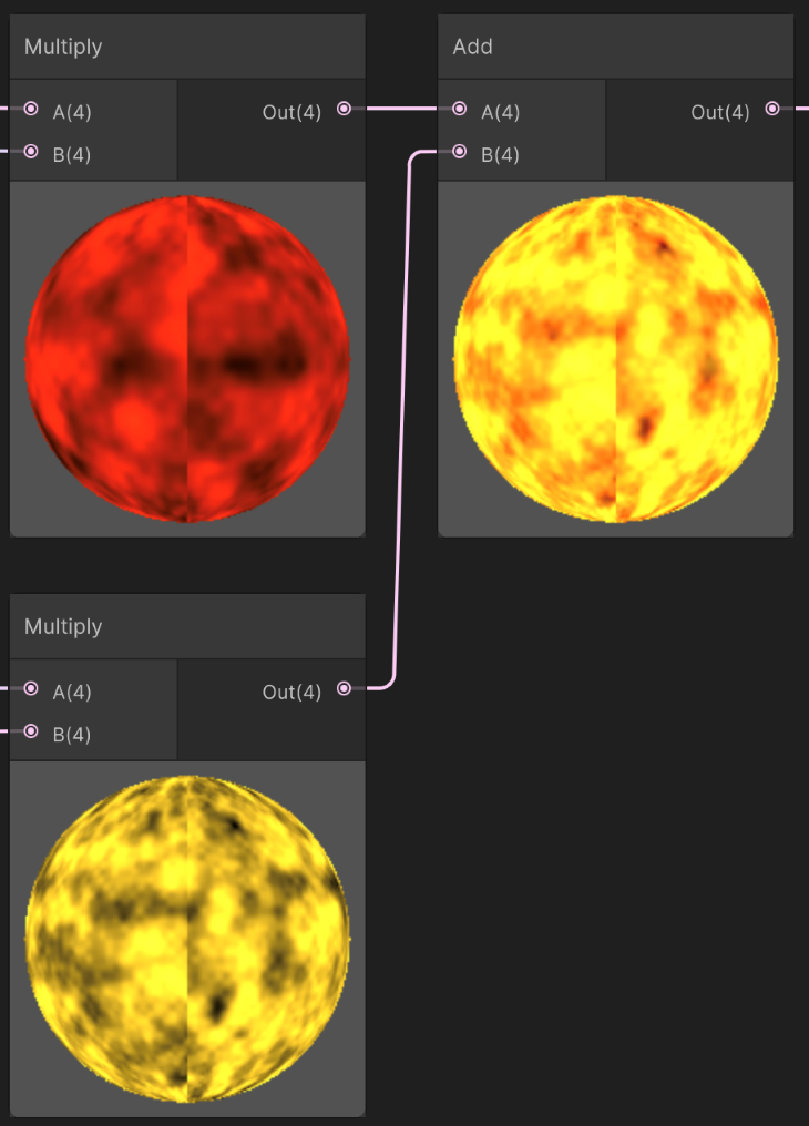
Both results are added together using the Add node. After combining them, we should already get a result resembling lava or a hot surface. To spice it further, we will add a pulsating color to emphasize the lava movement and fiery intensity.

For a more varied noise texture, we multiply both original noise results from the previous steps and use the result as the UV coordinates of a Voronoi Noise node. Mixing noise values and UV channels is a quick way of achieving a wide range of visuals.
Instead of using the resulting Voronoi directly, which would still be too similar to its inputs, we use the One Minus node to invert it, followed by a Saturate node that clamps the result between 0 and 1. The Saturate node is often used to guarantee that the result of inversion operations and other functions do not yield negative numbers that might cause issues with the upcoming nodes in the graph.
To select only isles from the current noise texture, we use the Step node again to filter only the results that are higher than a given value. For the result shown here, the value used was 0.33.
For the pulsating effect, we will oscillate the Angle Offset of the previously discussed Voronoi node by using a combination of the Time node and a Gradient Noise, as seen below.
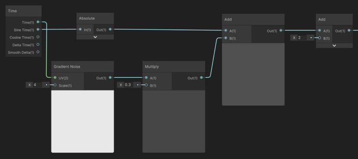
Generally, a good approach for pulsating values is to use the Sine or Cosine functions with the Time node. To save us some time, the Time node itself already contains outputs for both functions. As we do not want a negative pulse, we plug the sine value into an Absolute node.
To break the monotony of a simple sine function, we use a 1D Gradient Noise approach, by using the Time node output as a UV coordinate (thus, both x and y components are the same).
Notice that even though we are using a 1D result for the Gradient Noise node, it is important to still consider the scale input parameter. A larger value for the scale will cause more variation than a smaller one. In this scenario, we are using a scale of 4 to achieve a smaller variation over time.
Moreover, the Gradient Noise node output is multiplied by a value to control its intensity in the final result. This example multiplies it by 0.3 to reduce its impact to only 30 percent. Surely those values can be tweaked for a different desired outcome.
Finally, both the sine result and the noise are added up and used as the Angle Offset of the Voronoi Noise node.
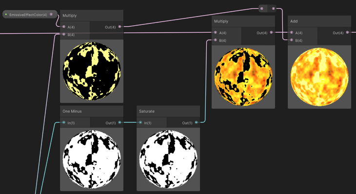
We take two steps to combine the pulsating colors into the previously lava texture we had.
The first one is to remove the pulsating area from the previously generated texture. If we ignore this step, adding (or multiplying) the pulsating value on top of the current result might alter the colors and results too much, either tending the result to a bland white color or canceling opposing colors (for example, if the pulse is Green and the texture is Blue).
An easy way to achieve the removal is to use again the One Minus node followed by a Satura node and multiply the result with the previous texture. That will make the pulsating area black and keep the non-pulsating area with its intended values.
Then, for the second step, we multiply the pulsating texture with the desired color and, using the Add node, add it to the last node, combining all of them.

As seen throughout this article, plenty of options enable noises and randomness in your Unity project. The standard math library and the Mathematics package allow various methods to use noise functions via code. At the same time, the Shader Graph tool provides three versatile noise function nodes for procedural generation.
Indeed, many other noise functions used by the industry are not entirely available through these methods, such as the Fractal Noise Function and the Curl Noise Function. However, most of those can be programmed in a C# function to be used in code or implemented in HLSL language in the Shader Graph. In other words, although not all functions are presented, we have enough tools to implement them.
Finally, consider that another easy alternative to the lack of specific noise functions or patterns is the use of premade textures. The Lava Flowing Shader is a free asset in Unity’s asset store that achieves a good-looking lava material by combining multiple textures and shader programming.
Consider that this discussion boils down to the usual conflict. At the same time, in developing applications, we can use more memory (textures) or more processing time (procedural noise functions) to achieve our results. It is up to us to decide what yields the best efficiency and workflow. Luckily enough, the noise functions presented have a minimal performance footprint.
Thanks for reading, and let me know if you would like more on Noise Functions, Shader Graph, and other fast development and prototyping techniques for Unity. You can see more of my work at www.dagongraphics.com.
Install LogRocket via npm or script tag. LogRocket.init() must be called client-side, not
server-side
$ npm i --save logrocket

// Code:

import LogRocket from 'logrocket';
LogRocket.init('app/id');
// Add to your HTML:

<script src="https://cdn.lr-ingest.com/LogRocket.min.js"></script>
<script>window.LogRocket && window.LogRocket.init('app/id');</script>

Learn how Vite+ unifies Vite, Vitest, Oxlint, Oxfmt, Rolldown, and Node.js management in one CLI.

AI companies are buying developer tools as coding agents turn runtimes, package managers, and linters into strategic infrastructure.
Learn how AI-assisted development governance uses rules, agents, hooks, and protocols to help AI coding tools produce safer, more consistent code.

A step-by-step guide to building your first MCP server using Node.js, covering core concepts, tool design, and upgrading from file storage to MySQL.
Hey there, want to help make our blog better?
Join LogRocket’s Content Advisory Board. You’ll help inform the type of content we create and get access to exclusive meetups, social accreditation, and swag.
Sign up now