Guide to using TensorFlow in Rust

TensorFlow, a powerful open source machine learning framework developed by the Google Brain team, has become a cornerstone in artificial intelligence. While traditionally associated with languages like Python, the advent of Rust, a systems programming language valued for its performance and safety, has opened new avenues for TensorFlow enthusiasts.

In this guide, we will explore the fusion of TensorFlow and Rust, delving into how we can integrate these two technologies to harness the strengths of both.

Setting up our TensorFlow boilerplate

All the code discussed in this article is available, and ready to run, in this GitHub repository. The boilerplate for TensorFlow is simple — add the following dependency in the Cargo.toml file:

[dependencies]
tensorflow = "0.21.0"

In case you want to use the GPU, just use the tensorflow_gpu feature in your Cargo.toml:

[dependencies]
tensorflow = { version = "0.21.0", features = ["tensorflow_gpu"] }

This is the only dependency we will need for the examples in the following sections. Just to verify that everything works, check the following program (you will find it in the directory tf-example1 in the repository):

extern crate tensorflow;

use tensorflow::Tensor;

fn main() {
    let mut x = Tensor::new(&[2]);
    
    x[0_usize] = 3.0f32;
    x[1_usize] = 2.0f32;

    println!("{:?}", x);
}

The program is simple but useful to check that everything is in place. Let’s take a deeper look at it. First we declare an external crate named tensorflow, indicating that the program will use the TensorFlow crate.

We then import the Tensor type from the TensorFlow crate. A tensor in TensorFlow represents a multidimensional array and is a fundamental data structure for computations. For a general introduction to TensorFlow concepts, you can refer to the official documentation.

The main function creates a new mutable tensor x with a one-dimensional vector with two elements. In TensorFlow, the shape of a tensor specifies the number of elements in each dimension: if you specify, for example, [2,3], the tensor will (unsurprisingly 🙂) have the shape of a 2×3 matrix.

Lastly, we just assign values to the elements of the tensor x. In this case, it sets the first element to 3.0 and the second element to 2.0. Finally, the program prints the tensor x using the println! macro. {:?} is a formatting specifier to print the tensor in a debug format.

Project overview and understanding the XOR function

Training a neural network to learn the XOR (exclusive OR) function is a classic example that highlights the capability of neural networks to learn complex relationships in data. XOR is a binary operation that outputs true (1) only when the number of true inputs is odd.

No matter how simple it is conceptually, the XOR example will help show us all the necessary steps to design, train, and use a model. Learning the XOR table of truth justifies the use of a hidden layer in the neural network; indeed, simpler networks, like a single neuron, cannot learn the XOR table of truth. So the XOR example is both simple to program and requires all the power of more complex neural networks.

The following code is in the directory tf-example2. The code has two functionalities, as you may expect: the training of the network, in the train function; and the inference, in the eval function. As an additional functionality, the training saves the trained model to let it be used later on.

Building our network with TensorFlow and Rust

Let’s get right into the code:

fn train<P: AsRef<Path>>(save_dir: P) -> Result<(), Box<dyn Error>> {
    // ================
    // Build the model.
    // ================
    let mut scope = Scope::new_root_scope();
    let scope = &mut scope;
    // Size of the hidden layer.
    // This is far more than is necessary, but makes it train more reliably.
    let hidden_size: u64 = 8;
    let input = ops::Placeholder::new()
        .dtype(DataType::Float)
        .shape([1u64, 2])
        .build(&mut scope.with_op_name("input"))?;
    let label = ops::Placeholder::new()
        .dtype(DataType::Float)
        .shape([1u64])
        .build(&mut scope.with_op_name("label"))?;
    // Hidden layer.
    let (vars1, layer1) = layer(
        input.clone(),
        2,
        hidden_size,
        &|x, scope| Ok(ops::tanh(x, scope)?.into()),
        scope,
    )?;
    // Output layer.
    let (vars2, layer2) = layer(layer1.clone(), hidden_size, 1, &|x, _| Ok(x), scope)?;
    let error = ops::sub(layer2.clone(), label.clone(), scope)?;
    let error_squared = ops::mul(error.clone(), error, scope)?;
    let mut optimizer = AdadeltaOptimizer::new();
    optimizer.set_learning_rate(ops::constant(1.0f32, scope)?);
    let mut variables = Vec::new();
    variables.extend(vars1);
    variables.extend(vars2);
    let (minimizer_vars, minimize) = optimizer.minimize(
        scope,
        error_squared.clone().into(),
        MinimizeOptions::default().with_variables(&variables),
    )?;

We begin by constructing a neural network model using TensorFlow. We must build the computation graph using Placeholder for input (the input variable) and target labels (the label variable).

In TensorFlow, a Placeholder serves as a variable to which data will be assigned when the Session begins (we’ll explore this in depth in the next section). This functionality allows the creation of processes or operations without an immediate need for data.

Then, two layers are created: a hidden layer (layer1) and an output layer (layer2). We do this with a handy function called layer that takes five input parameters:

1. The input layer (the layer to which we want to attach the new layer)
2. The size of the input layer
3. The output size (the number of new nodes we’ll create in the new layer)
4. The activation function of the newly created tensors
5. The scope within the new layer it will be created

// Returns variables created and the layer output.
fn layer<O1: Into<Output>>(
    input: O1,
    input_size: u64,
    output_size: u64,
    activation: &dyn Fn(Output, &mut Scope) -> Result<Output, Status>,
    scope: &mut Scope,
) -> Result<(Vec<Variable>, Output), Status> {
    let mut scope = scope.new_sub_scope("layer");
    let scope = &mut scope;
    let w_shape = ops::constant(&[input_size as i64, output_size as i64][..], scope)?;
    let w = Variable::builder()
        .initial_value(
            ops::RandomStandardNormal::new()
                .dtype(DataType::Float)
                .build(w_shape, scope)?,
        )
        .data_type(DataType::Float)
        .shape([input_size, output_size])
        .build(&mut scope.with_op_name("w"))?;
    let b = Variable::builder()
        .const_initial_value(Tensor::<f32>::new(&[output_size]))
        .build(&mut scope.with_op_name("b"))?;
    Ok((
        vec![w.clone(), b.clone()],
        activation(
            ops::add(
                ops::mat_mul(input, w.output().clone(), scope)?,
                b.output().clone(),
                scope,
            )?
            .into(),
            scope,
        )?,
    ))
}

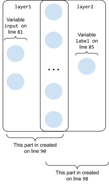
The result of calling the layer function is depicted in the following figure:

The first layer is created by calling the layer function using the Placeholder named input (containing two nodes) as the first parameter. This creates a subgraph that has two input nodes and an output layer containing hidden_size nodes (the left part of the figure below). The result is assigned to the object named layer1 to use in the next step of the construction.

The rightmost subgraph in the figure above is created by calling the layer function with the layer1 object as the first parameter. This will “stitch” the new layer on the rightmost part of layer1. The new layer will contain one single node: the output node for the whole network.

The activation function for the newly created tensors is tanh. You can see this by looking at the last parameter before scope where ops::tanh is passed as functional to the layer function; it is returned in the Ok value from the layer function. Together with the activation function, it also returns a vector containing all the tensors of the new layer.

As you can see, the layer function is quite handy and can be used iteratively to compose more complex graphs.

Training our network

After creating the network, we prepare SaveModelBuilder to be able to save the model once it is trained. For future reference, the model will be saved in the temporary directory on your disk — typically, it’s /tmp — and it will be named tf-rust-example-xor-saved-model.

The first step of the session is the initialization of all the variables. Before you can use operations in your model, you need to explicitly run variable initializers. The way we want to initialize our variable is set up by the layer function.

---

Over 200k developers use LogRocket to create better digital experiences

Learn more →

---

The explicit initialization is carried out by adding the invocation to the proper initializer op to the session. At this point, it is useful to explain the two concepts we are playing with in this code — graph and session:

• A graph outlines what computations to do. It doesn’t calculate anything or store values; it just describes the operations you wrote in your code. It is a static concept
• A session enables the execution of graphs or parts of them. It manages resources, possibly on multiple machines, and stores the real values of interim results and variables. It is a dynamic object that evolves

After setting up the initialization, we can start adding the proper training ops and execute the session. This is performed by another handy function, train, which is called 10,000 times. Let’s look at the train function:

    let mut train = |i| -> Result<f32, Box<dyn Error>> {
        input_tensor[0] = (i & 1) as f32;
        input_tensor[1] = ((i >> 1) & 1) as f32;
        label_tensor[0] = ((i & 1) ^ ((i >> 1) & 1)) as f32;
        let mut run_args = SessionRunArgs::new();
        run_args.add_target(&minimize);
        let error_squared_fetch = run_args.request_fetch(&error_squared, 0);
        run_args.add_feed(&input, 0, &input_tensor);
        run_args.add_feed(&label, 0, &label_tensor);
        session.run(&mut run_args)?;
        Ok(run_args.fetch::<f32>(error_squared_fetch)?[0])
    };

The train function takes an integer as input — the variable i — that is used to generate the input and the label for the graph. The input is prepared (intuitively, we take the first two bits of the i variable as input), and we calculate the label, which is the expected output of our network — in this case, of course, the XOR of the two input bits.

Then, the ops for feeding the graph and fetching the result are added at the session. The actual training is performed by executing the optimizer op that we added to the graph in the layer function.

Once the model is trained, we can save the model to reuse it later on without the need to retrain it. This is overkill for the XOR, but in general, it is always a good idea to save all the hard work for later.

Another point to discuss: the training here is made on a fixed number of training steps, but in the most general case, of course, you should adopt a different policy where you keep training as long as the error becomes smaller than a given threshold. Take a look at the following lines to get an idea of how to implement this:

    for i in 0..4 {
        let error = train(i)?;
        println!("Error: {}", error);
        if error > 0.1 {
            return Err(Box::new(Status::new_set(
                Code::Internal,
                &format!("Error too high: {}", error),
            )?));
        }
    }
    Ok(())

Evaluating our model

The evaluation of the training is carried out in the eval function, as you can see here:

fn eval<P: AsRef<Path>>(save_dir: P) -> Result<(), Box<dyn Error>> {
    let mut graph = Graph::new();
    let bundle = SavedModelBundle::load(
        &SessionOptions::new(),
        &["serve", "train"],
        &mut graph,
        save_dir,
    )?;
    let session = &bundle.session;
    let signature = bundle.meta_graph_def().get_signature(REGRESS_METHOD_NAME)?;
    let input_info = signature.get_input(REGRESS_INPUTS)?;
    let output_info = signature.get_output(REGRESS_OUTPUTS)?;
    let input_op = graph.operation_by_name_required(&input_info.name().name)?;
    let output_op = graph.operation_by_name_required(&output_info.name().name)?;

    let mut input_tensor = Tensor::<f32>::new(&[1, 2]);
    for i in 0..4 {
        input_tensor[0] = (i & 1) as f32;
        input_tensor[1] = ((i >> 1) & 1) as f32;
        let expected = ((i & 1) ^ ((i >> 1) & 1)) as f32;
        let mut run_args = SessionRunArgs::new();
        run_args.add_feed(&input_op, input_info.name().index, &input_tensor);
        let output_fetch = run_args.request_fetch(&output_op, output_info.name().index);
        session.run(&mut run_args)?;
        let output = run_args.fetch::<f32>(output_fetch)?[0];
        let error = (output - expected) * (output - expected);
        println!("Error: {}", error);
        if error > 0.1 {
            return Err(Box::new(Status::new_set(
                Code::Internal,
                &format!("Error too high: {}", error),
            )?));
        }
    }

    Ok(())
}

As you may expect, it’s nothing fancy. It simply loads the trained model we saved before and uses it to feed four integer numbers (once again, we will use the two less significative bits as inputs for the network) and fetch the result from the graph together with the calculated error.

First, we load the saved model; then, we recover, from the saved model bundle, the input and output operations from the graph. In the for loop, we assemble the input, feed it to the graph, and add the fetch operation.

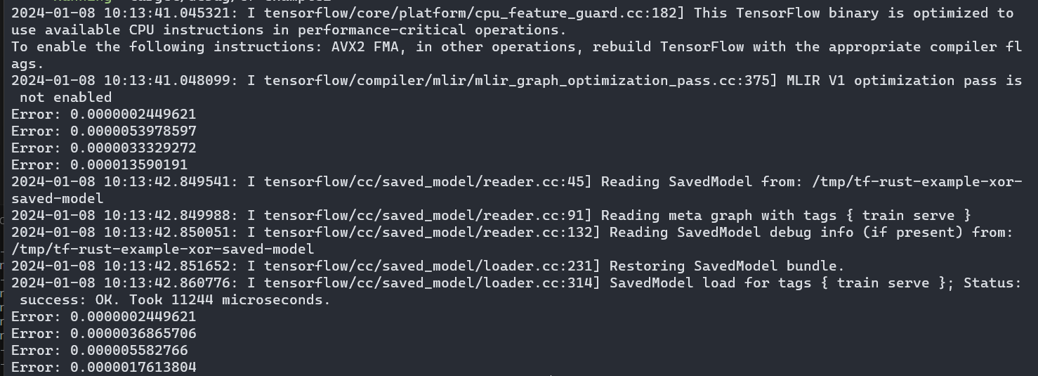
Once the session is run, we get the label from the output tensor and the calculated error between the value calculated from the model and the expected value we’ve calculated. You can see the output of the execution in the following figure:

Conclusion

In this article, we summarize two simple but relevant examples of using TensorFlow with Rust. The intent is to have an example simple enough not to get into the trouble of understanding complex models, yet complex enough to understand the concepts of building a network, training it, saving it, and loading the trained model.

LogRocket: Full visibility into web frontends for Rust apps

Debugging Rust applications can be difficult, especially when users experience issues that are hard to reproduce. If you’re interested in monitoring and tracking the performance of your Rust apps, automatically surfacing errors, and tracking slow network requests and load time, try LogRocket.

LogRocket lets you replay user sessions, eliminating guesswork around why bugs happen by showing exactly what users experienced. It captures console logs, errors, network requests, and pixel-perfect DOM recordings — compatible with all frameworks.

LogRocket's Galileo AI watches sessions for you, instantly identifying and explaining user struggles with automated monitoring of your entire product experience.

Modernize how you debug your Rust apps — start monitoring for free.